20  Model Selection and Validation

Reference: Chapter 5, [DM] Witten & Frank, Data Mining: Practical Machine Learning Tool and Techniques. (4th ed. 2017)

20.1 Why Evaluation

To determine which methods to use on a particular problem it is necessary a systematic way to evaluate how different methods work and compare one method with another one.

20.2 Issues in evaluation

Two main issues:

1. How to predict performance when a limited dataset is available

2. How to compare the performance of different ML algorithms on a given problem

20.3 Evaluation: ingredients

The ingredients are:

• Choice of performance measure (depending on the task to be solved) i.e.:
  • Number of correct classifications
  • Accuracy of probability estimates
  • Error in numeric predictions
• Costs assigned to different types of errors
  • Many practical applications involve costs
  • The cost of a misclassification error may depend on the type of error

20.4 Training and testing

For classification problems, it is natural to measure a classifier’s performance in terms of the error rate. The classifier predicts the class of each instance: if it is correct, that is counted as a success; if not, it is an error. The error rate is just the proportion of errors made over a whole set of instances.

Error rate on the training set is not likely to be a good indicator of future performance. Why? Because the classifier has been learned from the very same training data, any estimate of performance based on that data will be optimistic. The error rate on the training data is called the resubstitution error. Although it is not a reliable predictor of the true error rate on new data, it is nevertheless often useful to know.

To predict the performance of a classifier on new data, we need to assess its error rate on the test set. This is a dataset that never played any part in the training of the classifier. We assume that both the training data and the test data are representative samples of the underlying problem.

20.5 Making the most out of the data

If lots of data is available, there is no problem: we take a large sample and use it for training; then another, independent large sample of different data and use it for testing. Provided both samples are representative, the error rate on the test set will give a good indication of future performance. Generally, the larger the training sample the better the classifier, although the returns begin to diminish once a certain volume of training data is exceeded. And the larger the test sample, the more accurate the error estimate.

It may be that once the error rate has been determined, the test data (and validation data) is bundled back into the training data to produce a new classifier for actual use. There is nothing wrong with this: it is just a way of maximizing the amount of data used to generate the classifier that will actually be employed in production. This should not decrease predictive performance.

The real problem occurs when there is not a vast supply of data available. There’s a dilemma here: to find a good classifier, we want to use as much of the data as possible for training; to obtain a good error estimate, we want to use as much of it as possible for testing.

20.5.1 Holdout

The holdout method reserves a certain amount for testing, and uses the remainder for training (and sets part of that aside for validation, if required). Of course, you may be unlucky: the sample used for training (or testing) might not be representative. Each class in the full dataset should be represented in about the right proportion in the training and testing sets. If, by bad luck, all examples with a certain class were omitted from the training set, you could hardly expect a classifier learned from that data to perform well on examples of that class. Instead, you should ensure that the random sampling is done in a way that guarantees that each class is properly represented in both training and test sets. This procedure is called stratification, and we might speak of stratified holdout.

A more general way to mitigate any bias caused by the particular sample chosen for holdout is to repeat the whole process, training and testing, several times with different random samples. The error rates on the different iterations are averaged to yield an overall error rate. This is the repeated holdout method.

20.5.2 Cross validation

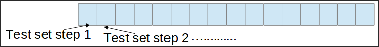
In a single holdout procedure, you might consider swapping the roles of the testing and training data reducing the effect of uneven representation in training and test sets. A simple variant forms the basis of an important technique called cross-validation.

In k-fold cross-validation, you decide on a fixed number of folds k of the data. Then the data is split into k subsets of (approximately) equal partitions: each in turn is used for testing and the remainder is used for training.

Often the subsets are stratified before the cross-validation is performed (stratified k-fold cross validation).

The error estimates are averaged to yield an overall error estimate.

The standard way of evaluation is to use stratified 10-fold cross-validation. Why 10? Extensive tests on numerous different datasets, with different learning techniques, have shown that 10 is about the right number of folds to get the best estimate of error, and there is also some theoretical evidence that backs this up. Neither the stratification nor the division into 10 folds has to be exact: it is enough to divide the data into 10 approximately equal sets in which the various class values are represented in approximately the right proportion.

A single 10-fold cross-validation might not be enough to get a reliable error estimate if the data is limited. Different 10-fold cross-validation experiments with the same learning scheme and dataset often produce different results, because of the effect of random variation in choosing the folds themselves. Stratification reduces the variance, but it certainly does not eliminate it entirely. When seeking an accurate error estimate with limited data, it is standard procedure to repeat the cross-validation process 10 times — i.e., 10 times 10-fold cross-validation and average the results.

20.5.3 Leave-One-Out

Leave-one-out cross-validation is simply n-fold cross-validation, where n is the number of instances in the dataset. Each instance in turn is left out, and the learning scheme is trained on all the remaining instances. It is judged by its correctness on the remaining instance. The results of all n judgments, one for each member of the dataset, are averaged, and that average represents the final error estimate.

This procedure is an attractive one for two reasons.

• The greatest possible amount of data is used for training in each case.

• The procedure is deterministic: no random sampling is involved. There is no point in repeating it 10 times, or repeating it at all: the same result will be obtained each time.

Set against this is the high computational cost, because the entire learning procedure must be executed n times and this is usually quite infeasible for large datasets. Additionally, it cannot be stratified. Stratification involves getting the correct proportion of examples in each class into the test set, and this is impossible when the test set contains only a single example.

Finally, imagine a completely random dataset that contains exactly the same number of instances of each of two classes. The best that an inducer can do with random data is to predict the majority class, giving a true error rate of 50%. But in each fold of leave-one-out, the opposite class to the test instance is in the majority (we have removed one instance) — and therefore the predictions will always be incorrect, leading to an estimated error rate of 100%!

20.5.4 Bootstrap

The bootstrap method is based on the statistical procedure of sampling with replacement.

The idea of the bootstrap is to sample the dataset with replacement to form a training set. A dataset of n instances is sampled n times, with replacement, to give another dataset of n instances. Because some elements in this second dataset will be repeated, there must be some instances in the original dataset that have not been picked: we will use these as test instances.

The chance that a particular instance will not be picked for the training set is \dfrac{1}{n}. So its probability of ending up in the test data is

\left(1 - \dfrac{1}{n} \right)^n \approx e^{-1} = 0.368

For a reasonably large dataset the test set will contain about 36.8% of the instances and the training set will contain about 63.2% of them. Some instances will be repeated in the training set, bringing it up to a total size of n, the same as in the original dataset.

The true error rate over the test set will be a pessimistic estimate, because the training set contains only 63% of the instances. To compensate for this, we combine the test set error rate with the resubstitution error on the instances in the training set as follows:

e = 0.632 \cdot e_{\text{test instances}} + 0.368 \cdot e_{\text{training instances}}

Then, the whole bootstrap procedure is repeated several times, with different replacement samples for the training set, and the results averaged.

The bootstrap procedure may be the best way of estimating error for very small datasets. However it has disadvantages that can be illustrated by considering a particular situation: a completely random dataset with two classes of equal size. The true error rate is 50% for any prediction rule. But a scheme that memorized the training set would give a perfect resubstitution score of 100%, so that e_\text{training instances} = 0, and the 0.632 bootstrap will mix this in with a weight of 0.368 to give an overall error rate of only 31.6% (0.632 \cdot 50% + 0.368 \cdot 0%), which is misleadingly optimistic, but still better than the leave-one-out estimation.

20.6 Hyperparameter selection

Many learning algorithms have parameters that can be tuned. These are called hyperparameters to distinguish them from basic parameters such as the coefficients in linear regression models. Best performance on a test set is achieved by adjusting the value of this hyperparameter to suit the characteristics of the data. However it is very important not to use performance on the test data to choose the best value for k! This is because peeking at the test data to make choices automatically introduces optimistic bias in the performance score. Instead, we split the original training set into a smaller, new training set and a validation set. The split is done randomly. Then the algorithm is run several times with different hyperparameter values on this reduced training set, and each of the resulting models is evaluated on the validation set. Once the hyperparameter value that gives best performance on the validation set has been determined, a final model is built by running the algorithm with that hyperparameter value on the original, full training set (train + val).

When applying the above parameter selection process multiple times within a cross-validation, once for each fold, it is possible that the hyperparameter values will be slightly different from fold to fold. This does not matter: what is being evaluated with cross-validation is the learning process, not one particular model.

There is a drawback to this process for hyperparameter selection: if the original training data is small then splitting off a validation set will further reduce the size of the set available for training. This means that the choice of hyperparameter may not be reliable. This is analogous to the problem with the simple holdout estimate, and the same remedy applies: use cross-validation instead. This means that a inner cross-validation is applied to determine the best value of the hyperparameter for each fold of the outer cross-validation used to obtain the final performance estimate for the learning algorithm. This kind of nested cross-validation process is expensive and it is common practice to use a smaller number of folds for the internal cross-validation.

20.7 Predicting performance: statistically estimate the error

The idea is to estimate the interval of confidence that an algorithm has a certain accuracy.

In statistics, a succession of independent events that either succeed or fail is called a Bernoulli process. Imagine that there is a Bernoulli process, like a biased coin, whose true (but unknown) success rate is p.

Suppose that out of N trials, S are successes: thus the observed success rate is f = \dfrac{S}{N}. We can say that p lies within a certain specified interval with a certain specified confidence (confidence interval).

20.7.1 Estimating confidence interval

20.7.1.1 The idea

The mean and variance of a single Bernoulli trial with success rate p are p and p(1-p), respectively. If N trials are taken from a Bernoulli process, the expected success rate f = \dfrac{S}{N} is a random variable with the same mean p; the variance is reduced by a factor of N to \dfrac{p(1-p)}{N}. For large N, the distribution of this random variable approaches the normal distribution. The probability that a random variable X, with zero mean, lies within a certain confidence range of width 2z is

P(-z \leq X \leq z) = c

With a symmetric distribution, like the normal one:

P(-z \leq X \leq z) = 1 - 2 \cdot P(X \geq z)

20.7.1.2 The method

All we need to do now is reduce the random variable f to have zero mean and unit variance. We do this by subtracting the mean p and dividing by the standard deviation \sqrt{\dfrac{p(1 - p)}{N}}. This leads to

P \left( -z < \dfrac{f - p}{\sqrt{\dfrac{p(1-p)}{N}}} < z \right) = c

Solving for p gives the upper and lower bound of the confidence interval:

p = \dfrac{\left( f + \frac{z^2}{2N} \pm z \sqrt{\frac{f}{N} - \frac{f^2}{N} + \frac{z^2}{4N^2}} \right)} { \left( 1 + \frac{z^2}{N} \right)}

20.8 Comparing learning schemes

It is important to determine whether one scheme is really better than another on a particular problem and demonstrate that the improvement is not just by chance.

Significance tests tell us how confident we can be that there is really a difference between the two learning schemas. What we want to determine is whether one scheme is better or worse than another on average, across all possible training and test datasets that can be drawn from the domain.

20.8.1 Assumptions

For now we assume that the supply of data is unlimited and suppose that cross-validation is being used to obtain the error estimates (other estimators, such as repeated cross-validation, are equally viable). For each learning scheme we can draw several datasets of the same size, obtain an accuracy estimate for each dataset using cross-validation, and compute the mean of the estimates. Each cross-validation experiment yields a different, independent error estimate. What we are interested in is the mean accuracy across all possible datasets of the same size, and whether this mean is greater for one scheme or the other.

20.8.2 Paired t-test

From this point of view, we are trying to determine whether the mean of a set of samples — cross-validation estimates for the various datasets that we sampled from the domain — is significantly greater or significantly less than the mean of another. This is a job for the Student’s t-test. Because the same cross-validation experiment can be used for both learning schemes to obtain a matched pair of results for each dataset, a more sensitive version of the t-test known as a paired t-test can be used.

There is a set of samples x_1, x_2, …, x_k obtained by k-fold cross-validations using one learning scheme, and a second set of samples y_1, y_2, …, y_k obtained by k-fold cross-validations using the other learning scheme. Each cross-validation estimate is generated using a different dataset (but all datasets are of the same size and from the same domain). We will get best results if exactly the same cross-validation partitions are used for both schemes, so that x_1 and y_1 are obtained using the same cross-validation split, as are x_2 and y_2, and so on. Denote the mean of the first set of samples by \overline{x} and the mean of the second set by \overline{y}. We are trying to determine whether \overline{x} is significantly different from \overline{y}.

If there are enough samples, the mean of a set of independent samples has a normal distribution. However, the variance is unknown, and the only way we can obtain it is to estimate it from the set of samples. The variance of x can be estimated by dividing the variance calculated from the samples x_1, x_2, …, x_k — call it \sigma^2_x — by k. We can reduce the distribution of \overline{x} to have zero mean and unit variance by using

\dfrac{\overline{x} - \mu}{\dfrac{\sigma_x}{\sqrt{k}}}

where \mu is the true value of the mean.

Because the variance is only an estimate, this does not have a normal distribution (although it does become normal for large values of k). Instead, it has a Student’s distribution with k-1 degrees of freedom.

To decide whether the means \overline{x} and \overline{y}, each an average of the same number k of samples, are the same or not, we consider the differences d_i between corresponding observations, d_i = x_i - y_i. This is legitimate because the observations are paired. The mean of this difference is just the difference between the two means, \overline{d} = \overline{x} - \overline{y}, and it has a Student’s distribution with k-1 degrees of freedom. If the means are the same (no “real” difference), the difference is zero (null hypothesis); if they’re significantly different, the difference will be significantly different from zero. So for a given confidence level, we will check whether the actual difference exceeds the confidence limit.

First, reduce the difference to a zero mean, unit variance variable called the t-statistic:

t = \dfrac{\overline{d}}{\sqrt{\dfrac{\sigma^2_d}{k}}}

where \sigma^2_d is the variance of the difference samples. Then, decide on a confidence level.

A two-tailed test is appropriate because we do not know in advance whether the mean of the x’s is likely to be greater than that of the y’s or vice versa: thus for a 1% test we use the value corresponding to 0.5%. If the value of t according to the formula above is greater than z, or less than -z, we reject the null hypothesis that the means are the same and conclude that there really is a significant difference between the two learning methods on that domain for that dataset size.

20.8.3 Nonpaired t-test

What if we were unable to assess the error of each learning scheme on the same datasets?

What if the number of datasets for each scheme was not even the same?

For instance, we used k estimates for one scheme, and j estimates for the other one.

Then it is necessary to use a nonpaired t-test. The t-statistic becomes

t = \dfrac{\overline{d}}{\sqrt{\dfrac{\sigma^2_x}{k} + \dfrac{\sigma_y^2}{j}}}

The degrees of freedom should be taken conservatively to be the minimum of the degrees of freedom of the two samples: in this way we are sure that the value of t is not underestimated, because a lower value of degrees of freedom corresponds to a higher value of z for the same confidence level, and so a higher value of t is required to reject the null hypothesis.

20.8.4 The real case

In practice there is usually only a single dataset of limited size. We could split the data into subsets and perform a cross-validation on each one. However, the overall result will only tell us whether a learning scheme is preferable for that particular size. Alternatively, the original dataset could be reused with different randomizations of the dataset for each cross-validation. However, the resulting cross-validation estimates will not be independent because they are not based on independent datasets. Just increasing the number of samples k, for instance increasing the number of cross-validation runs, will eventually yield an apparently significant difference because the value of the t-statistic increases without bound.

Heuristic modifications of the standard t-test have been proposed to circumvent this problem. One that appears to work in practice is the corrected resampled t-test.

Each time, n_1 instances are used for training and n_2 for testing, and differences d_i are computed from performance on the test data. The corrected resampled t-test uses the modified statistic

t = \dfrac{\overline{d}}{\sqrt{\left(\dfrac{1}{k} + \dfrac{n_2}{n_1}\right) \sigma_d^2}}

A closer look at the formula shows that its value cannot be increased simply by increasing k.

The same modified statistic can be used with repeated cross-validation: for 10-fold cross-validation repeated 10 times, k = 100, \dfrac{n_2}{n_1} = \dfrac{0.1}{0.9}, and \sigma^2_d is based on 100 differences.

20.9 Predicting Probabilities

Throughout this section we have tacitly assumed that the goal is to maximize the success rate of the predictions and the outcome for each test instance is either correct or incorrect. This is called 0-1 loss:

L(y, \hat{y}) = \begin{cases} 0 & \text{if } y = \hat{y} \\ 1 & \text{if } y \neq \hat{y} \end{cases}

However, most learning schemes produces class probabilities, we might want to check the accuracy of the probability estimates. It might be more natural to take this probability into account when judging correctness to evaluate the confidence that the learning schema has about the prediction. In this case, 0-1 loss is not the right measure because we lose the information provided by the probabilities.

20.9.1 When to use prediction probabilities

If the ultimate application is just a prediction of the outcome, and no prizes are awarded for a realistic assessment of the likelihood of the prediction, it does not seem appropriate to use probabilities. If the prediction is subject to further processing, however then it may well be appropriate to take prediction probabilities into account.

20.9.2 Quadratic loss function

Suppose for a single instance there are k possible outcomes, or classes, and for a given instance the learning scheme comes up with a probability vector. The actual outcome for that instance will be one of the possible classes.

However, it is convenient to express it as a vector a_1, a_2 , …, a_k whose ith component, where i is the actual class, is 1 and all other are 0. We can express the penalty associated with this situation as a loss function that depends on both p and a using the quadratic loss:

\sum_j (p_j - a_j)^2 = \sum_{j \neq c} p_j^2 + (1 - a_c)^2

This is for a single instance, when the test set contains several instances, the loss function is summed over them all. The goal is to minimize E[\sum_j (p_j - a_j)^2], it can be shown that this is minimized when the probability estimate p_i = p_i^*:

E\left[\sum_j (p_j - a_j)^2\right] = \sum_j \left(E[p_j^2] - 2E[p_j a_j] + E[a_j^2]\right) = \sum_j (p_j^2 - 2p_j p_j^* + p_j^{*2}) = \sum_j \left((p_j - p_j^*)^2 + p_j^*(1-p_j^*)\right)

The first stage just involves bringing the expectation inside the sum and expanding the square. For the second, p_j is just a constant and the expected value of a_j is p_j^*; moreover, because a_j is either 0 or 1, a^2_j = a_j and its expected value is p^*_j too. The third stage is straightforward algebra. To minimize the resulting sum, it is clear that it is best to choose p_j = p_j^*. If the true probabilities are unknown the minimization will be given by the best estimate of p_c.

20.9.3 Informational loss function

Another criterion is the informational loss function:

-\log_2 p_i

where p_i is the probability of the actual class. It represents the information in bits required to express the actual class with respect to the probability distribution.

The expected value of the informational loss function, if the true probabilities are p_1^*, p_2^*, …, p_k^*, is

-p_1^* \log_2 p_1 - p_2^* \log_2 p_2 - \ldots - p_k^* \log_2 p_k

This expression is minimized by choosing p_j = p_j^*, in which case the expression becomes the entropy of the true distribution:

-\sum_j p_j^* \log_2 p_j^*